Research
Statistical Model of Nonharmonic Internal Tides
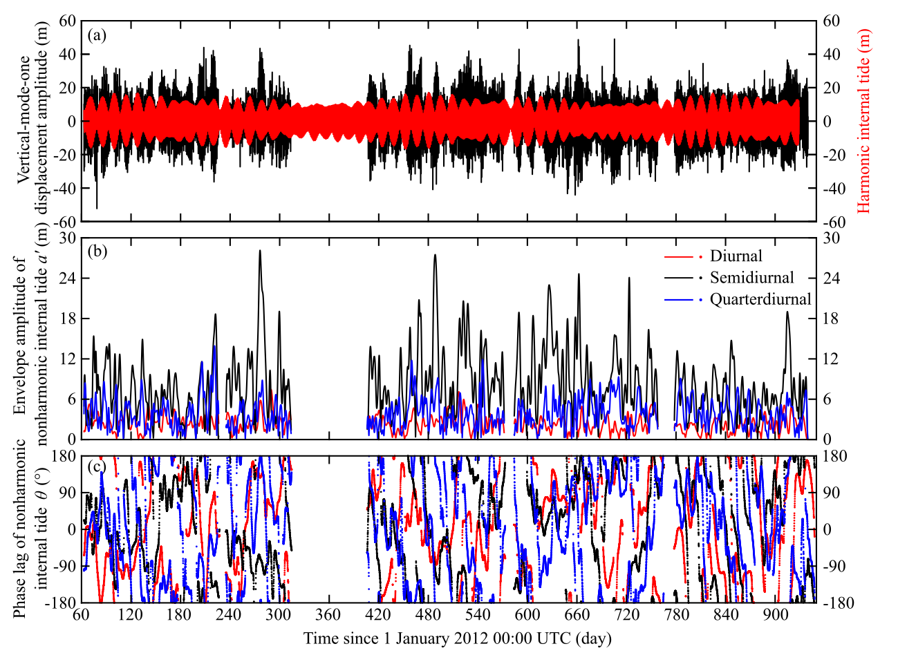
Fig. 1. Time series of variables related to vertical-mode-one internal tides from PIL200 observations. (a) Isopycnal displacement amplitude and its harmonic component, and (b, c) envelope amplitudes and phase lags of diurnal, semi-diurnal, and quarter-diurnal components of nonharmonic internal tides.
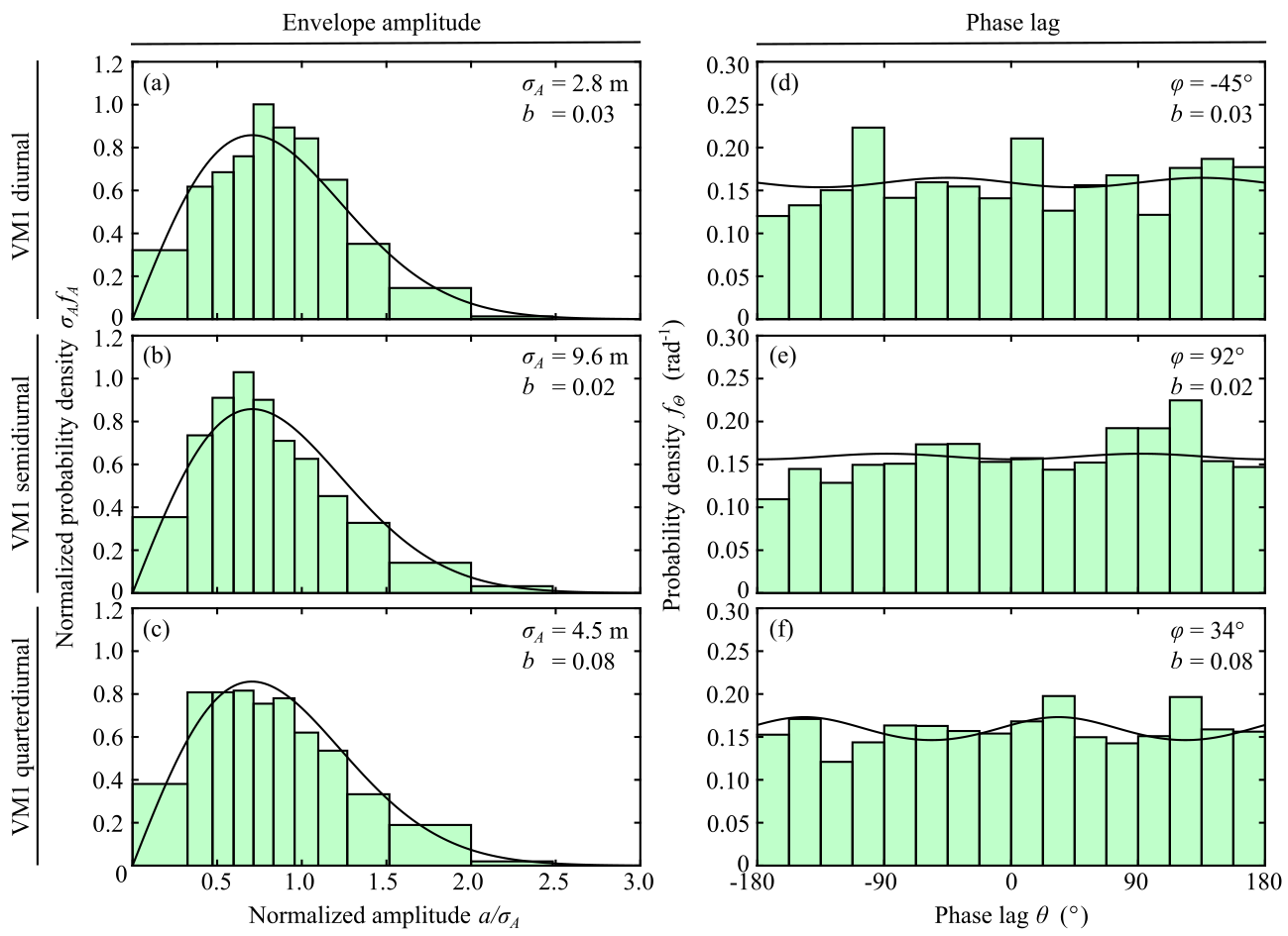
Fig. 2. Comparisons of envelope-amplitude and phase probability density functions from the statistical model and PIL200 observations for nonharmonic vertical-mode-one internal tides. (a–c) Envelope amplitude, (d–f) phase lag. Upper, middle, and bottom rows show diurnal, semi-diurnal, and quarter-diurnal components, respectively. Solid lines show distributions in the “many source” limit, with estimated model parameters shown in each panel.
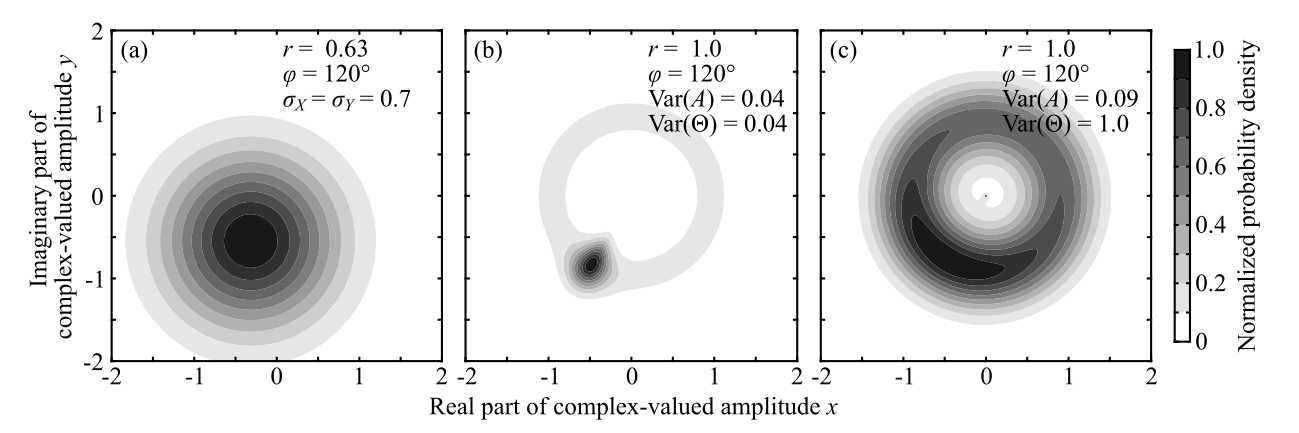
Fig. 3. Comparison of probability density functions (PDFs) under simple (or “toy”) models. (a) PDF under Eq. \eqref{simpleModelNew}, (b) PDF under Eq. \eqref{simpleModelPrevious} with relatively small $\text{Var}(A)$ and $\text{Var}(\Theta)$, and (c) that under relatively large $\text{Var}(A)$ and $\text{Var}(\Theta)$. The parameters used are shown in each panel.
Motivation
Internal tides are internal waves at tidal frequencies generated by the interaction of usual (barotropic) tides and topographic slopes. However, they are known to contain substantial components that cannot be predicted by (deterministic) harmonic analysis, because random oceanic variability modulates their amplitudes and phases. Although the statistical aspects of these random nonharmonic components are important basis for many purposes, they have not been considered in detail. This study develops the first detailed statistical model of nonharmonic (also called incoherent, nonstationary, or non-phase-locked) internal tides observed at a fixed location.
Theoretical model
Since it is well-known that internal tides at an observation location can consist of waves arriving from multiple and remote sources4,5), it is expected from the central limit theorem in statistics that the process becomes Gaussian as the number of wave sources increases. As a model of nonharmonic internal tides, we consider a sinusoidal signal with a constant angular frequency $\omega$, a random amplitude $A$, and a random phase lag $\Theta$ observed at a fixed location, and assume that this signal consists of independent and non-uniformly distributed sinusoidal signals from many sources. This can be written as \begin{align} A\text{e}^{-\text{i}\Theta}\text{e}^{\text{i}\omega t} &=(X+\text{i} Y)\text{e}^{\text{i}\omega t}\\ &= \sum_{j=1}^N (X_j+\text{i} Y_j) \text{e}^{\text{i}\omega t}, \end{align} where $t$ is time, $(X+\text{i} Y)$ is the Cartesian representation of the complex-valued amplitude $A\text{e}^{-\text{i}\Theta}$, and $N$ is the number of wave components (sources). If $N$ is sufficiently large, and if $X$ and $Y$ are independent, the PDF approaches the joint Gaussian distribution. By writing it in polar coordinates, we get the amplitude PDF $f_A$ and the phase PDF $f_\Theta$: \begin{align} f_{A}(a)&\sim\dfrac{2a}{\sigma_{A}^2\sqrt{1-b^2}}\exp\left(-\dfrac{a^2}{(1-b^2)\sigma_{A}^2}\right)I_0\left(\dfrac{ba^2}{(1-b^2)\sigma_{A}^2}\right),\\ f_{\Theta}(\theta)&\sim \dfrac{1}{2\pi}\dfrac{\sqrt{1-b^2}}{1-b\cos 2(\theta-\varphi)},\\ \sigma_{A}^2&=\sigma_{X}^2+\sigma_{Y}^2,\\ b&=\sigma_{A}^{-2}|\sigma_{X}^2-\sigma_{Y}^2|. \end{align} Here, $\sigma_{X}^2$ and $\sigma_{Y}^2$ are respectively the variance of $X$ and $Y$, $\varphi$ is the mean phase lag, and $I_0$ is the modified Bessel function of the first kind of the order 0.
Observations
To test the applicability of the above statistical model, we compared the model PDFs with observed PDFs at the PIL200 location (of Australian IMOS) on the Australian North West Shelf. The observations were made at about 200-m water depth over about 2.5 years. The data were processed as follows.
- Estimated amplitudes of the dominant internal-wave mode, called vertical mode one, at 15-min intervals (black line in Fig. 1a).
- Calculated harmonic internal tides by applying harmonic analysis to the whole record (red line in Fig. 1a).
- Calculated nonharmonic internal tides by subtracting the harmonic internal tides from the original amplitudes.
- Extracted envelope amplitudes and phase lags for the diurnal (24 h), semi-diurnal (12 h), and quarter-diurnal (6h) components by band-pass filtering (Fig. 1c,d).
Results
The model PDFs were statistically not different from the observed PDFs for both envelope amplitudes and phases for the diurnal, semi-diurnal, and quarter-diurnal nonharmonic internal tides (Fig. 2).
Discussion
To my knowledge, this is the first study that developed a detailed statistical model of nonharmonic internal tides. The statistical information, such as the amplitude PDF, provides an important basis for many purposes, as seen in the example of surface waves for engineering applications.
The results of this study may appear trivial because it follows from the central limit theorem; however, this is the first study that showed the importance of viewing nonharmonic internal tides as the superposition of many wave components. For example, previous studies considered one wave-component model in which the amplitude and phase are normally distributed1,2): \begin{align} \label{simpleModelPrevious} \eta=(r+A) \text{e}^{\text{i}(\omega t-\Theta)}.\tag{1} \end{align} Here, $\eta$ is the displacement amplitude of internal tides, and $r$ is the harmonic amplitude. However, this study suggests that the corresponding simple model in many wave-component case is \begin{align} \label{simpleModelNew} \eta=r \text{e}^{\text{i}(\omega t-\varphi_0)}+(X+\text{i} Y) \text{e}^{\text{i}(\omega t-\varphi)},\tag{2} \end{align} where $X$ and $Y$ are normally distributed. Since \eqref{simpleModelPrevious} has to assume small $A$, a broad Gaussian form from \eqref{simpleModelNew} (Fig. 3a) cannot be represented by \eqref{simpleModelPrevious} (Fig. 3b,c). The difference can be important because \eqref{simpleModelPrevious} has been used to analyse observed nonharmonic internal tides1-3, 6), but this study suggests that \eqref{simpleModelNew} is likely to be more appropriate.
Finally, this study unfortunately suggests difficulty in process investigation of nonharmonic internal tides based on their observations at one location, because their variability and PDFs tend to approach the universal form by statistical principles, regardless of the details of individual wave components. For process investigation, the proposed statistical model was used to develop a model suite for Combined Adjoint, Statistical, and Stochastic Modelling of Nonharmonic Internal Tides.
Related Publications
Details of this study are available in
The data from the above study are available in
Acknowledgements
The PIL200 data were sourced from the Australian Integrated Marine Observing System (IMOS) – IMOS is a national collaborative research infrastructure, supported by the Australian Government. I thank Jonas Nycander for his suggestion to simplify the derivation of the statistical model.
References
- Colosi, J. A. and Munk, W. 2006. Tales of the venerable Honolulu tide gauge. Journal of Physical Oceanography, 36: 967–996, https://doi.org/10.1175/JPO2876.1.
- Geoffroy, G. and Nycander, J. 2022. Global mapping of the nonstationary semidiurnal internal tide using Argo data. Journal of Geophysical Research - Oceans, 127: e2021JC018283, https://doi.org/10.1029/2021JC018283.
- Kachelein, L., Gille, S. T., Mazloff, M. R., and Cornuelle, B. D. 2024. Characterizing non-phase-locked tidal currents in the California Current system using high-frequency radar, Journal of Geophysical Research - Oceans, 129: e2023JC020340, https://doi.org/10.1029/2023JC020340.
- Ponte, A. L. and Cornuelle, B. D. 2013. Coastal numerical modelling of tides: Sensitivity to domain size and remotely generated internal tide. Ocean Modelling, 62: 17–26, https://doi.org/10.1016/j.ocemod.2012.11.007.
- Rainville, L., Johnston, T. M. S., Carter, G. S., Merrifield, M. A., Pinkel, R., Worcester, P. F., and Dushaw, B. D. 2010. Interference pattern and propagation of the M2 internal tide south of the Hawaiian Ridge. Journal of Physical Oceanography, 40: 311–325, https://doi.org/10.1175/2009JPO4256.1.
- Zaron, E. D. 2022. Baroclinic tidal cusps from satellite altimetry. Journal of Physical Oceanography, 52: 3123–3137, https://doi.org/10.1175/JPOD- 21-0155.1.