Research
Analytical Models of Capped Turbulent Oscillatory Bottom Boundary Layers
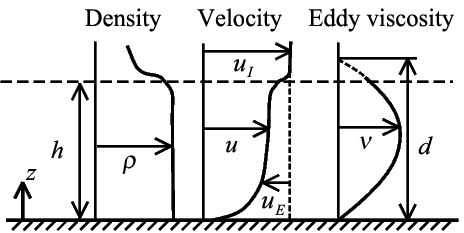
Fig. 1. Schematic of a capped bottom boundary layer and definition of variables. Figure taken from Shimizu (2010, J. Geophys. Res.-Oceans).
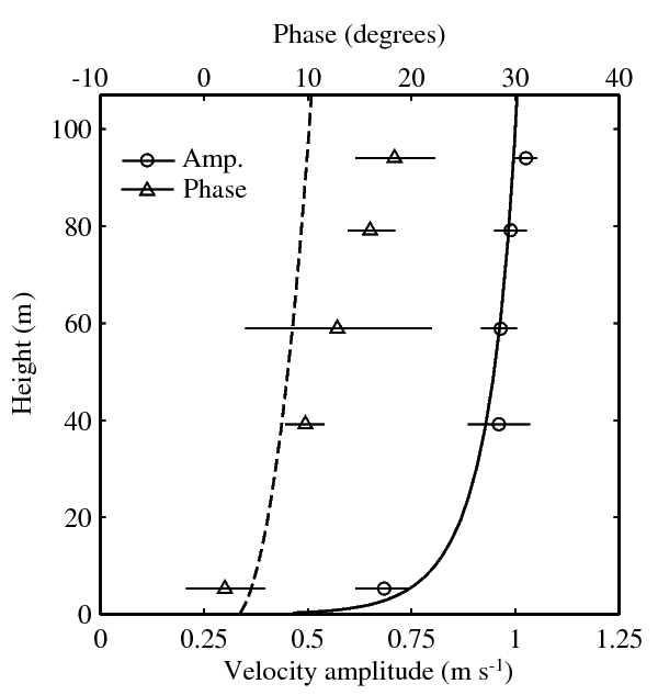
Fig. 2. Comparison with a M2 tidal current profile at Admiralty Inlet, Washington, USA. Symbols show data from Mofjeld and Lavelle (1984) with the horizontal bars representing 99% confidence intervals. Lines are the best fit of the proposed theory. Figure taken from Shimizu (2010, J. Geophys. Res.-Oceans).
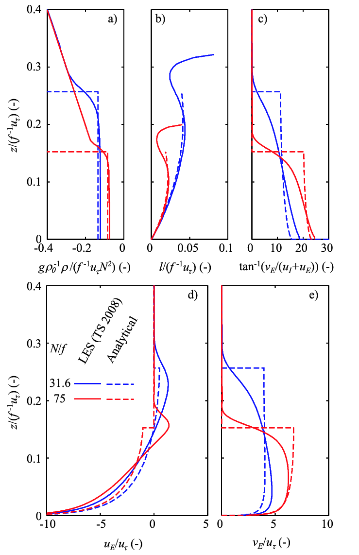
Fig. 3. Comparison with caped Ekman layer solutions computed by Taylor and Sarkar (2008). Vertical profiles of normalized (a) density, (b) mixing length, (c) veering angle, and velocities (d) parallel and (e) normal to the interior flow. $g$ is the acceleration due to gravity, and $N$ is the buoyancy frequency. Reformatted from Shimizu (2010, J. Geophys. Res.-Oceans).
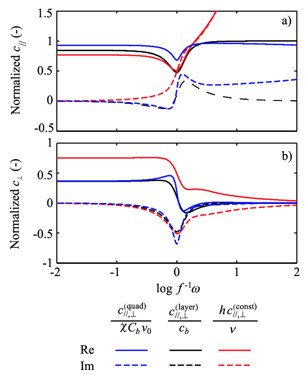
Fig. 4. Comparison of normalized friction coefficients $c_{//}$ and $c_{\perp}$ from different boundary-layer models under typical conditions in Lake Kinneret in summer. $c^{(quad)}_{//,\perp}$ and $c^{(const)}_{//,\perp}$ are friction coefficients for vertically dependent models with quadratic (proposed) and constant eddy viscosity. $c^{(layer)}_{//,\perp}$ are friction coefficients from the layer-averaged model. Reformatted from Shimizu and Imberger (2010, Limnol. Oceanogr.).
Motivation
An analytical model of bottom boundary layers (BBLs) provides not only an conceptual understanding of the dynamics, but also bottom boundary conditions for the far-field flow. In oceans and lakes, bottom-generated turbulence tends to create a well-mixed BBL capped by a sharp density gradient at the top. To include the effects of this capping, the use of quadratic eddy viscosity was proposed for turbulent bottom Ekman layers2),3). By applying this suggestion to rotating oscillatory BBLs, I proposed a new analytical model of capped turbulent oscillatory BBLs. Then, I used the model to develop a simpler, layer-averaged linear BBL model, which can be used in modal analysis for semi-enclosed basins (see examples for Lake Biwa and Lake Kinneret).
A Quadratic-Eddy-Viscosity Model
Fig. 1 shows the idealized capped BBL used for this study and the definition of relevant variables. The governing equations for the Ekman part of the velocity $\vec{v}_E=(u_E, v_E)$ are7)
\begin{equation} \frac{\partial \vec{v}_E}{\partial t} = - f \vec{k} \times \vec{v}_E + \frac{\partial}{\partial z} \left( \kappa z \left( 1-\frac{z}{d} \right) u_\tau \frac{\partial \vec{v}_E }{\partial z} \right), \end{equation}where $f$ is the Coriolis parameter, $\vec{k}$ is the vertical unit vector, and $u_\tau$ is the friction velocity. We assume an oscillatory interior flow
\begin{equation} \vec{v}_I=\frac{1}{2}\tilde{\vec{v}}_I e^{\mathrm{i} \omega t} + c.c., \end{equation}where $\omega$ is the angular frequency, and $c.c.$ represents the complex conjugate of the preceding term. The solution has the form:
\begin{equation} \begin{bmatrix} u_E \\ v_E \end{bmatrix} = -\frac{1}{2} \begin{bmatrix} H_{//} & -H_{\perp} \\ H_{\perp} & H_{//} \end{bmatrix} \begin{bmatrix} \tilde{u}_I \\ \tilde{v}_I \end{bmatrix} e^{\mathrm{i} \omega t} + c.c., \end{equation}where $H_{//}$ and $H_{\perp}$ are vertical structure functions. Although this model is conceptually simple, the solution is unfortunately a bit difficult to handle because $H_{//}$ and $H_{\perp}$ are written in terms of the hypergeometric functions $_2F_1$ with complex-valued arguments. One of the important parameters coming out of the BBL model is the bottom shear stress
\begin{equation} \begin{bmatrix} \tau_x \\ \tau_y \end{bmatrix} = \frac{\rho_0}{2} \begin{bmatrix} c_{//} & -c_{\perp} \\ c_{\perp} & c_{//} \end{bmatrix} \begin{bmatrix} \tilde{u}_I \\ \tilde{v}_I \end{bmatrix} e^{\mathrm{i} \omega t} + c.c., \end{equation}where $\rho_0$ is the reference density, and $c_{//}$ and $c_{\perp}$ are two complex-valued friction coefficients calculated from $H_{//}$ and $H_{\perp}$.
Choosing the friction velocity $u_\tau$ provides a 'closure' to this nonlinear problem. Since I was interested in applying this model to damping of internal waves, I proposed to choose $u_\tau$ such that the model yields the correct average dissipation rate over a period. The common choice of $u_\tau$ based on maximum shear stress was found unsatisfactory for rotating flows from an energetics point of view.
Comparisons with Field Data and Simulation results
- Comparison with the observation of M2 tidal currents in a narrow open channel1) (Fig. 2). The magnitude is predicted well by the theory; however, the phase varies only half as much as the measurements, which is a known limitation of time-independent eddy viscosity models8).
- Comparison with Large Eddy Simulation (LES) of capped Ekman layers6) (Fig. 3). The velocity profiles are not predicted well; however, the parameters important for setting bottom boundary conditions, e.g., the bottom shear stress, veering angle at the bottom, and Ekman transport, are predicted well by the theory.
Reduction to A Layer-Averaged BBL Model
The quadratic-eddy-viscosity model was used to develop a simpler layer-averaged BBL model that is compatible with modal analysis for semi-enclosed basins. This layer-averaged BBL model is based on
\begin{align} \frac{\partial \vec{v}_E}{\partial t} = f \vec{k} \times \vec{v}_E - \frac{1}{\rho h} \vec{\tau}, \\ \vec{\tau} = \chi C_b v_0 \left( \vec{v}_I + \vec{v_E} \right), \end{align}where $C_b$ is the usual drag coefficient, and $v_0$ is the typical interior velocity. Note that the flow is allowed to slip at the top of the BBL. The model constant $\chi$ is introduced to minimize the difference in energy dissipation rate between this layer-averaged model and the quadratic-eddy-viscosity model. The layer-averaged model show frequency characteristics different from capped BBLs with constant eddy viscosity, but similar to those with quadratic eddy viscosity (Fig. 4).
Related Publications
Details of the quadratic-eddy-viscosity model are available in
The layer-averaged BBL model for modal analysis is described in
Acknowledgements
I appreciate Sutanu Sarker for kindly providing the original LES results presented in Taylor and Sarkar (2008) to plot a figure.
References
- Mofjeld, H. O., and J. W. Lavelle. 1984. Setting the length scale in a second-order closure model of the unstratified bottom boundary layer. Journal of Physical Oceanography, 14: 833–839.
- Perlin, A., J. N. Moum, J. M. Klymak, M. D. Levine, T. Boyd, and P. M. Kosro. 2005. A modified law-of-the-wall applied to oceanic bottom boundary layers. Journal of Geophysical Research - Oceans, 110: C10S10, doi:10.1029/2004JC002310.
- Perlin, A., J. N. Moum, J. M. Klymak, M. D. Levine, T. Boyd, and P. M. Kosro. 2007. Organization of stratification, turbulence, and veering in bottom Ekman layers. Journal of Geophysical Research - Oceans, 112: C05S90, doi:10.1029/2004JC002641.
- Shimizu, K. 2010. An analytical model of capped turbulent oscillatory bottom boundary layers. Journal of Geophysical Research – Oceans, 115: C03011. doi:10.1029/2009JC005548.
- Shimizu, K., and J. Imberger. 2010. Seasonal differences in the evolution of damped internal waves in a stratified lake. Limnology and Oceanography, 57: 1449-1462.
- Taylor, J. R., and S. Sarkar. 2008. Stratification effects in a bottom Ekman layer. Journal of Physical Oceanography, 38: 2535–2555.
- Weatherly, G. L., and P. J. Martin. 1978. On the structure and dynamics of the oceanic bottom boundary layer. Journal of Physical Oceanography, 8: 557–570.
- Zou, Q. 2002. An analytical model of wave bottom boundary layers incorporating turbulent relaxation and diffusion effects, Journal of Physical Oceanography, 32: 2441– 2456