Research
Adjoint Frequency Response Analysis
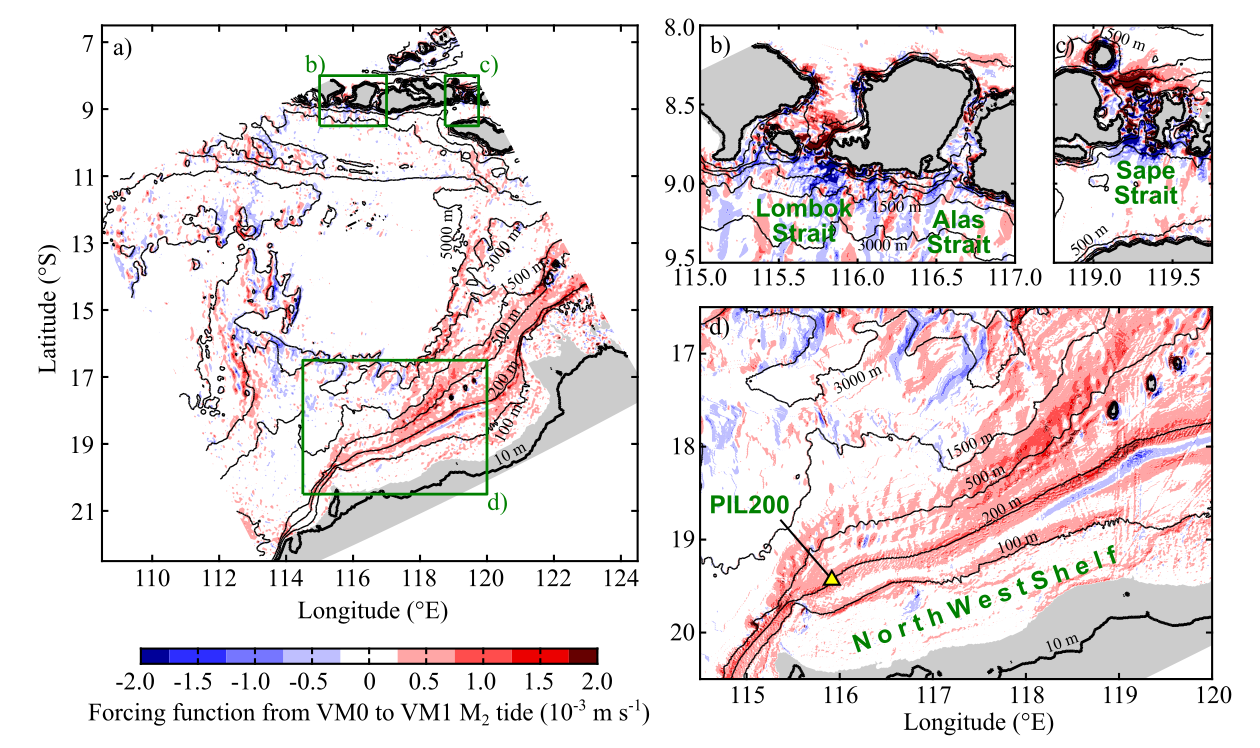
Fig. 1. Forcing function from the barotropic-mode (VM0) to vertical-mode-one (VM1) M2 tide (at zero Greenwich phase lag). It corresponds to $\tilde{\boldsymbol{f}}$ in \eqref{objectiveFunFT}. Panel (a) shows the whole model domain, and panels (b)–(d) show zoomed views of the green boxes in (a). Grey shading shows regions where VM1 celerity is less than 0.1 m/s.
Fig. 2. Adjoint frequency response function of vertical-mode-one (VM1)-induced isopycnal displacement at the PIL200 location to M2 tidal forcing at other locations (at zero Greenwich phase lag). It corresponds to $\tilde{\boldsymbol{\lambda}}$ in \eqref{objectiveFunFT}.
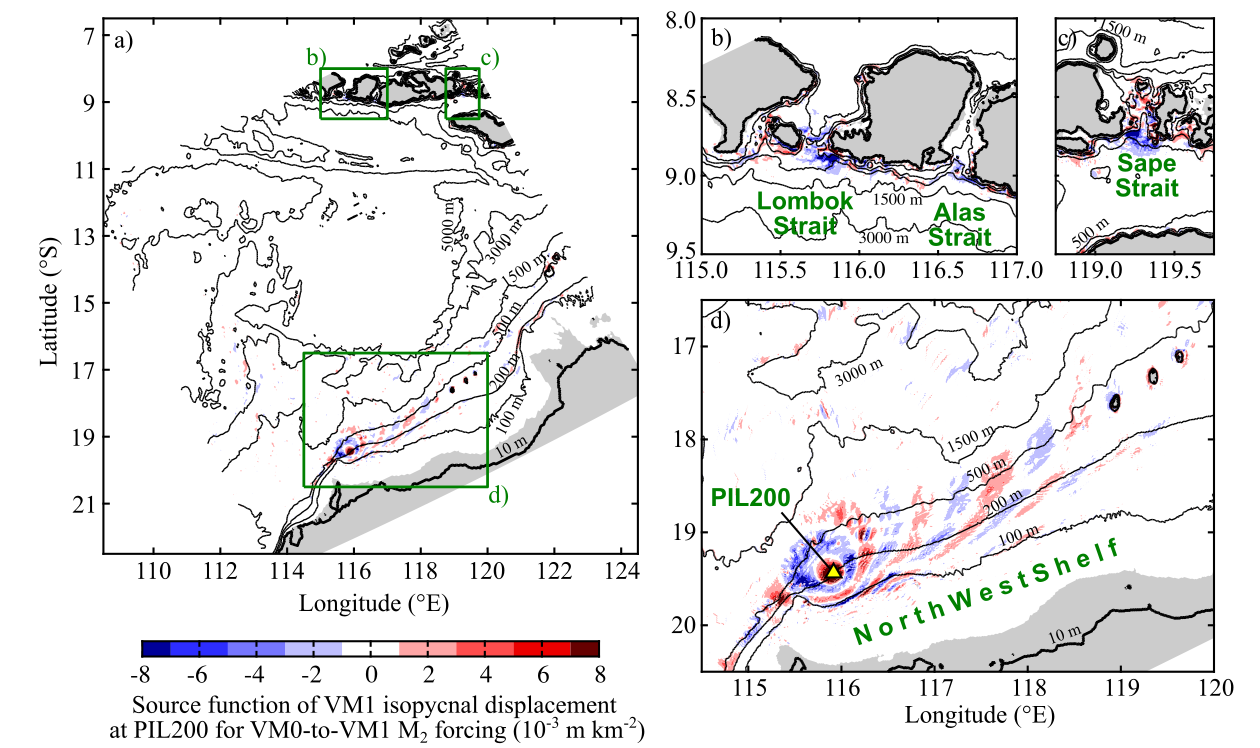
Fig. 3. Source function of vertical-mode-one (VM1)-induced isopycnal displacement at the PIL200 location for M2 tidal forcing (at zero Greenwich phase lag). It corresponds to each element of $\tilde{\boldsymbol{\lambda}}^H\tilde{\boldsymbol{f}}$ before the sum in \eqref{objectiveFunFT}. Panel (a) shows the whole model domain, and panels (b)–(d) show zoomed views of the green boxes in (a).
Motivation
The adjoint method is a common technique used in inverse problems. It provides the sensitivity of an arbitrary variable of interest, called objective or cost function, to the model input data. In oceanography, it is often used in so-called four-dimensional variational (4D-Var) data assimilation for forecasts and reanalysis1,3), but it has other potential applications. This study explores a new application of the adjoint method for mapping the sources of periodic phenomena, such as tides.
Theory
We consider a linear model:
\begin{align} \label{linearModel} \dfrac{\partial \boldsymbol{x}}{\partial t}=&-\mathbf{L}\boldsymbol{x}+\boldsymbol{f},\tag{1} \end{align}where $\boldsymbol{x}(t)$ is the model state vector containing the model's prognostic variables, $\mathbf{L}$ is the matrix operator representing the linear dynamics, and $\boldsymbol{f}(t)$ is the external forcing. The objective function defined at $t=t_j$ can be written as2)
\begin{align} J(t_j) =& \boldsymbol{w}^H\boldsymbol{x}(t)\\ =&\int_{-\infty}^{t_j}\boldsymbol{\lambda}^H(t_j-\tau)\boldsymbol{f}(\tau)\text{d}\tau,\label{objectiveFun} \tag{2} \end{align}where $\boldsymbol{w}$ is the time-independent weight vector used to define $J$, $()^H$ denotes conjugate transpose, and $\boldsymbol{\lambda}$ is the sensitivity of $J$ to $\boldsymbol{x}$. $\boldsymbol{\lambda}$ can be calculated from the adjoint of \eqref{linearModel}:
\begin{align} -\dfrac{\partial \boldsymbol{\lambda}}{\partial t}=&-\mathbf{L}^H\boldsymbol{\lambda},\\ \boldsymbol{\lambda}=&\boldsymbol{w}\quad\text{at}\quad t=t_j. \end{align}If we now allow $t_j$ to vary and consider time-dependent $J$, the Fourier transform of \eqref{objectiveFun} is
\begin{align} \label{objectiveFunFT} \tilde{J}(\omega)=\tilde{\boldsymbol{\lambda}}^H(\omega)\tilde{\boldsymbol{f}}(\omega) \tag{3} \end{align}because \eqref{objectiveFun} is convolution. Here, $\omega$ is the angular frequency. This is convenient because we can consider the forcing $\tilde{\boldsymbol{f}}$ and dynamic response $\tilde{\boldsymbol{\lambda}}$ separately, and the result is their product. Furthermore, since the total $\tilde{J}$ is given by the vector sum, the vector elements corresponding individual grid points can be used to produce maps.
An example application to VM1 internal tides at PIL200 location
To illustrate the application of adjoint frequency response analysis, the method is applied to internal tides observed at PIL200 location (of Australian IMOS) on the Australian North West Shelf. We focus on the dominant mode of internal tides, called vertical mode one (VM1).
Fig. 1 shows the forcing function from the usual (barotropic) tides to VM1 internal tides, corresponding to $\tilde{\boldsymbol{f}}$ in \eqref{objectiveFunFT}. This map is obtained using tidal currents and background stratification, which are model inputs. It shows "global" forcing applicable to any locations.
Fig. 2 shows the adjoint frequency response function calculated by numerical modelling. It corresponds to $\tilde{\boldsymbol{\lambda}}$ in \eqref{objectiveFunFT}. The alternating colour corresponds to the phase of internal tides. The magnitude decays with distance mostly due to spreading.
Fig. 3 shows the source function. This map is obtained by the element-wise multiplication of $\tilde{\boldsymbol{f}}$ in Fig. 1 and $\tilde{\boldsymbol{\lambda}}^H$ in Fig. 2. Unlike the forcing function, the source function shows only sources relevant for internal tides at the PIL200 location. Note that there are relatively small regions with significant magnitudes, such as the Australian shelf around the PIL200 location and the straits in Indonesian archipelago.
Discussion
The adjoint frequency response analysis has several important advantages.
- It yields information that is relevant to the location and variable of interest. For internal tides, the existence of many sources and wide propagation directions make it difficult to obtain such information from the usual hydrodynamic modelling.
- The results can be presented as simple maps. For example, Fig. 3 can be used to visually identify important sources regions. This is useful for planning field measurements and improving model performance by data assimilation.
- Sources distribution in Fig. 3 turned out to be useful for stochastic modelling of the random components of internal tides, as described in Combined Adjoint, Statistical, and Stochastic Modelling of Nonharmonic Internal Tides.
Related Publications
Details of this study are available in
The data from the above study are available in
Acknowledgements
The original idea of the adjoint frequency response analysis was developed while I was at the Max Planck Institute for Meteorology under the financial support of the Max Planck Society for the Advancement of Science through the Klaus Hasselmann Postdoctoral Fellowship. I thank Jochem Marotzke for the introduction to adjoint modelling.
References
- Bennett, A. F. 2002. Inverse Modeling of the Ocean and Atmosphere, Cambridge University Press.
- Marotzke, J., R. Giering, K. Q. Zhang, D. Stammer, C. Hill, and T. Lee. 1999. Construction of the adjoint MIT ocean general circulation model and application to Atlantic heat transport sensitivity. J. Geophys. Res.: Oceans, 104, 29529-29547.
- Wunsch, C. 2006. Discrete inverse and state estimation problems. Cambridge University Press.