Research
Combined Adjoint, Statistical, and Stochastic Modelling of Nonharmonic Internal Tides
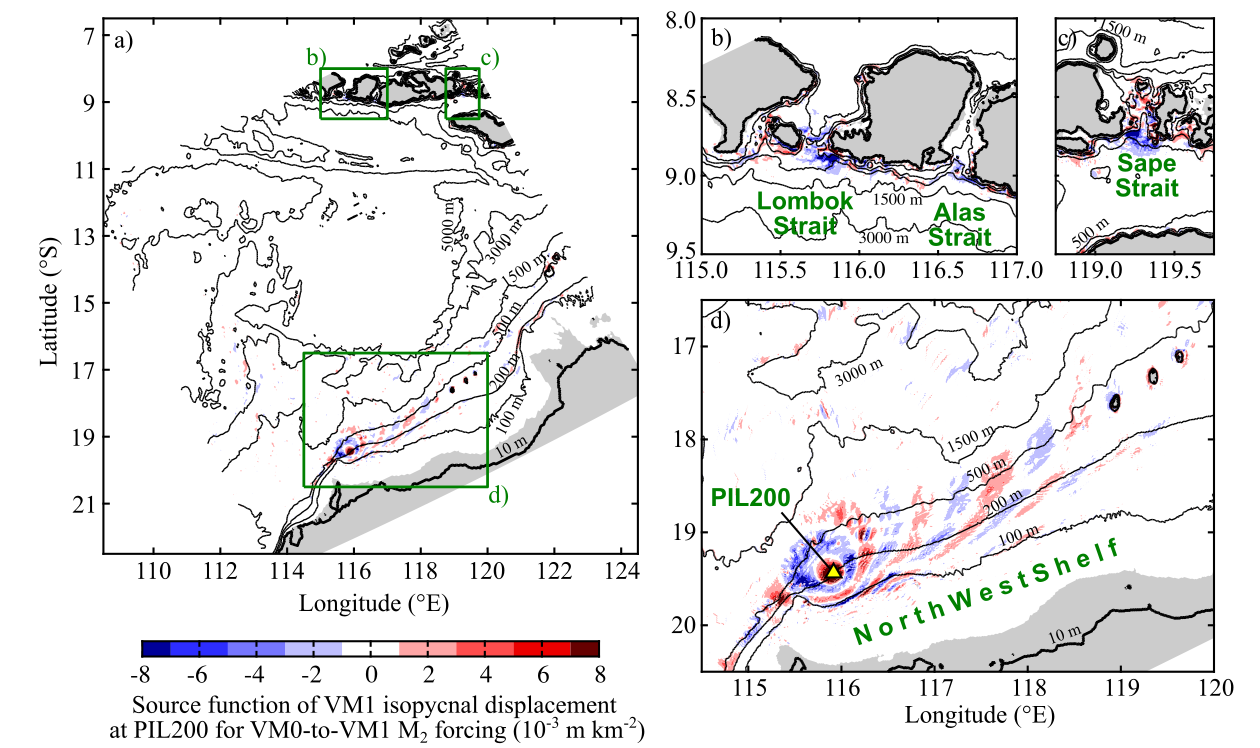
Fig. 1. Source function of vertical-mode-one (VM1)-induced isopycnal displacement at the PIL200 location for M2 tidal forcing (at zero Greenwich phase lag). Panel (a) shows the whole model domain, and panels (b)–(d) show zoomed views of the green boxes in (a). Grey shading shows regions where celerity is less than 0.1 m/s.
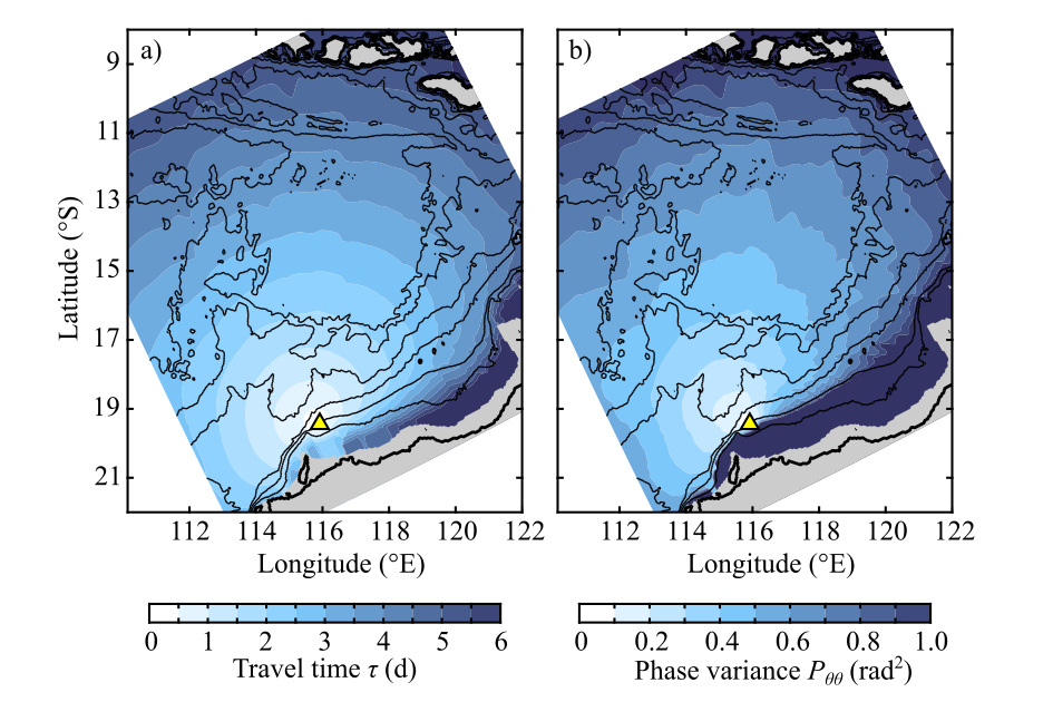
Fig. 2. Maps of variables related to the phase modulation of a vertical-mode-one semi-diurnal internal tide at the PIL200 location in the reference case. (a) Travel time, and (b) phase variance. Yellow triangles indicate the PIL200 location.
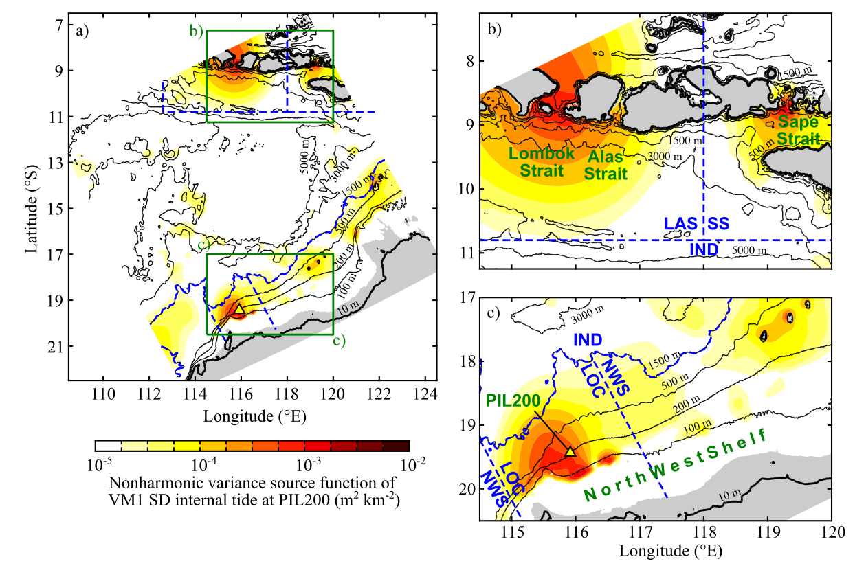
Fig. 3. Nonharmonic variance source function of isopycnal displacement induced by the nonharmonic vertical-mode-one (VM1) semi-diurnal (SD) internal tide at the PIL200 location in the reference case. The four major semi-diurnal constituents are included. Panel (a) shows the whole model domain, and panels (b)–(d) show zoomed views of the green boxes in (a).
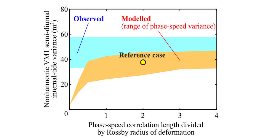
Fig. 4. Dependence of the nonharmonic vertical-mode-one (VM1) semi-diurnal internal tide at the PIL200 location on phase-speed variance $\sigma_C^2$ and the ratio of phase-speed correlation length $L_C$ to the Rossby radius of deformation.
Table 1 Contributions of different regions to nonharmonic vertical-mode-one semi-diurnal internal-tide variance at the PIL200 location in the reference case. The regions are defined in Fig. 3.
| Region | Integrated variance contribution (m2) |
|---|---|
| LOC | 6.0 |
| NSW | 8.2 |
| LAS | 13.5 |
| SS | 2.6 |
| IND | 7.5 |
| Total | 37.8 |
Motivation
Internal tides are internal waves at tidal frequencies generated by the interaction of usual (barotropic) tides and topographic slopes. However, they are known to contain substantial random components that cannot be predicted by (deterministic) harmonic analysis. For random nonharmonic internal tides originating from distributed sources, the superposition of many waves with different degrees of randomness unfortunately makes process investigation difficult. This study develops a new model suite for process-based modelling of nonharmonic internal tides by combining adjoint, statistical, and stochastic approaches, and applies it to internal tides at the PIL200 location (of Australian IMOS) on the Australian North West Shelf for process investigation.
Methods
Statistical model
Statistical Model of Nonharmonic Internal Tides provides the basis of the model suite. An internal tide signal is assumed to have a random amplitude $A$ and a random phase $\Theta$ at an observation location, which results from the superposition of many independent waves with deterministic amplitudes $a_j$ and random phases $\Theta_j$:
\begin{align} A\text{e}^{-\text{i}(\varphi+\Theta)}\text{e}^{\text{i}\omega t} = \sum_{j=1}^N a_j \text{e}^{-\text{i}(\varphi_j+\Theta_j)} \text{e}^{\text{i}\omega t}. \end{align}Here, $t$ is time, $\omega$ is the angular frequency, $\varphi$ and $\varphi_j$ are the mean phase lags, and $N$ is the number of sources. The variance of this signal is
\begin{align} \text{E}\left(A^2\right)&=\boldsymbol{s}^H\mathbf{\Sigma}^{2}\boldsymbol{s}, \end{align}where $\boldsymbol{s}$ a vector containing the deterministic complex-valued amplitudes $a_j\text{e}^{-\text{i}\varphi_j}$, and $\mathbf{\Sigma}^2$ is a diagonal matrix whose diagonal elements are $(1-\text{e}^{-\sigma_j^2})$, where $\sigma_j^2=\text{Var}(\Theta_j)$. The components of the right-hand-side before the sum can be used to produce the source map of nonharmonic internal-tide variance. The modelling of $\text{E}\left(A^2\right)$ requires $\boldsymbol{s}$ and $\sigma_j^2$, which are modelled as follows.
(It is also essential to consider correlated sources, but it is omitted here. Please see my paper listed below for the details.)
Adjoint model
Adjoint Frequency Response Analysis was used to calculate deterministic wave amplitudes at the sources $\boldsymbol{s}$. The resulting $\boldsymbol{s}$ for VM1 M2 internal tide is shown in Fig. 1.
Stochastic model
Zaron and Egbert4) showed that the phase variance $\sigma_j^2$ can be related to the variability of the internal-tide phase speed $c_j$. This leads to the stochastic differential equations (SDEs):
\begin{align} \text{d}c_j'&=-\dfrac{\overline{c}_j}{L_C}c_j'\text{d}t+\sqrt{\dfrac{\overline{c}_j}{L_C}}\text{d}b_j,\\ \text{d}\theta_j&=-\dfrac{\omega c_j'}{\overline{c}_j}\text{d}t. \end{align}Here, $\theta_j$ is the stochastic version of $\Theta_j$, and $\overline{c}_j$ and $c_j'$ are the mean and deviation deviation of $c_j$, $L_C$ is the phase-speed correlation length, and $\text{d}b_j$ contains white noise. Because the above two equations are linear SDEs, the variance equations associated with them are3)
\begin{align} \dfrac{\text{d} P_{c\theta}}{\text{d} t}&=-\dfrac{\overline{c}}{L_C}P_{c\theta}-\dfrac{\omega}{\overline{c}}\sigma_C^2,\\ \dfrac{\text{d} P_{\theta\theta}}{\text{d} t}&=-2\dfrac{\omega}{\overline{c}}P_{c\theta}, \end{align}where $P$ denotes the covariance between two variables shown in the subscript, and $\sigma_C^2$ is the phase-speed variance. We integrate these equations along wave propagation paths calculated by the standard ray theory2). The resulting $P_{\theta\theta}=\sigma_j^2$ for VM1 M2 internal tide is shown in Fig. 2.
Synthesis
The above modelling was done for the four major semi-diurnal tidal constituents (M2, S2, K2, N2). The resulting total variance is compared to the observed semi-diurnal variance.
Results
The source map of nonharmonic internal-tide variance shows two particularly important source regions: the Australian shelf and the straits in Indonesian archipelago (Fig. 3). The total modelled nonharmonic internal-tide variance using reference $\sigma_C^2$ and $L_C$ is 38 m2 compared to the observed variance of 45 ± 12 m2.
The contributions of different regions defined in Fig. 3 show the relative importance of remote sources (Table 1). This is because it takes time for internal tides to be modulated by oceanic variability (Fig. 2b).
The parameter dependence of modelled nonharmonic internal-tide variance on $\sigma_C^2$ and $L_C$ (Fig. 4) shows that it is essential to consider phase-speed correlation, and that the modelled variance is consistent with the observation for the realistic parameter range of $L_C$ > (Rossby radius of deformation).
Discussion
This study developed a completely new model suite useful for process investigation. Also, the source map (Fig. 3) was shown to be a new convenient tool to identify important source regions of nonharmonic internal tides. This is useful for planning field measurements and improving model performance by data assimilation.
In terms of processes, this study added further support that the phase modulation process is caused by phase-speed variability along deterministic (or mean) propagation paths4) as a first approximation. The phase-speed correlation length was found to be important parameters controlling the nonharmonic internal-tide variance, in addition to phase-speed variance which has been identified in previous studies1,4).
Since this is a feasibility study of the proposed new model suite, there are many aspects of the model suite that can evolve in the future. The most important caveat appears to the use of ray theory to calculate internal-tide propagation path.
Related Publications
Details of this study are available in
The data from the above study are available in
References
- Buijsman, M. C., Arbic, B. K., Richman, J. G., Shriver, J. F., Wallcraft, A. J., and Zamudio, L. 2017. Semidiurnal internal tide incoherence in the equatorial Pacific, Journal of Geophysical Research - Oceans, 122: 5286–5305, https://doi.org/10.1002/2016JC012590.
- Lighthill, J. 1978. Waves in Fluids, Cambridge University Press.
- Särkkä, S. and Solin, A. 2019. Applied Stochastic Differential Equations, Cambridge University Press.
- Zaron, E. D. and Egbert, G. D. 2014. Time-variable refraction of the internal tide at the Hawaiian Ridge. Journal of Physical Oceanography, 44: 538–557, https://doi.org/10.1175/JPO-D-12-0238.1.