Research
Properties of Adjoint Model and Adjoint Sensitivity under Fully-Nonlinear Internal Waves
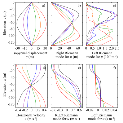
Fig.1. Semi-analytic solution for 1st-baroclinic-mode right-propagating simple internal wave and associated Riemann modes. Selected (a-c) isopycnal-displacement and (d-f) horizontal-velocity profiles and corresponding right and left Riemann modes. Also see additional figure panel here.
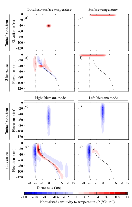
Fig.2. Comparisons of adjoint MITgcm outputs under different choices of objective function. Forward model state is infinitely long, strongly nonlinear internal wave field. First and third rows show "initial" adjoint sensitivity to temperature, set by the objective function. Second and fourth rows show corresponding sensitivity three hours earlier in the adjoint model. Dotted and dashed lines indicate horizontal displacements caused by wave propagation and advection, respectively.

Fig. 3. Adjoint sensitivity of simple-wave amplitude (Riemann variable) $R$ at x ~ 33 km to temperature under semi-diurnal internal waves. (a) "Initial" condition, (b) 5 hrs earlier, and (c) 10 hrs earlier. Black lines show 22 to 30°C isotherms from the forward model at 2°C intervals. Click image to see the movie (1.0MB, not for small screen).
Motivation
Adjoint sensitivity modeling is a common technique used to solve inverse problems, including so-called four-dimensional variational (4D-Var) data assimilation used in weather forecasts and ocean reanalysis1,5). It provides the sensitivity of an objective (or cost) function to the model input data. Although the model resolution has become often high enough to resolve internal tides in ocean modelling, it remains unclear whether physically-sensible adjoint sensitivity modeling is feasible in the presence of internal waves. As a first step to tackle this problem, this study investigates fundamental properties of the adjoint of a time-dependent circulation model, and the resulting sensitivity under internal waves.
Theory
Since adjoint sensitivity under internal waves has not been investigated before, it is important to understand properties of the adjoint model and resulting sensitivity theoretically. The essential aspects can be understood using the shallow water equations, which is the forward model of this example: \begin{align} \dfrac{\partial\boldsymbol{p}}{\partial t}&=-\boldsymbol{K}\dfrac{\partial\boldsymbol{p}}{\partial x}, \\ \partial\boldsymbol{p}&=\begin{bmatrix}\eta\\u\end{bmatrix}, \\ \boldsymbol{K}(\boldsymbol{p})&=\begin{bmatrix}u&H+\eta\\c^2 H^{-1}&u\end{bmatrix}. \end{align} Here, $x$ is the horizontal coordinate, $t$ is the time, $\eta(x,t)$ is the surface displacement, $u(x,t)$ is the (vertically uniform) horizontal velocity, $H$ is the (constant) water depth at equilibrium, $c=\sqrt{gH}$ is the propagation speed of long linear surface gravity waves, and $g$ is the acceleration due to gravity. Assuming that the objective (or cost) function $j^\text{sens}$ (one of the model inputs) is defined at the end of the forward model run at $t=t_j$, the adjoint of the shallow water equation is \begin{align} \dfrac{\partial}{\partial t}\left(\dfrac{\partial j}{\partial\boldsymbol{p}}\right)&=-\boldsymbol{K}^T\dfrac{\partial}{\partial x}\left(\dfrac{\partial j}{\partial\boldsymbol{p}}\right),\\ \left(\dfrac{\partial j}{\partial\boldsymbol{p}}\right)&=\left(\dfrac{\partial j^\text{sens}}{\partial\boldsymbol{p}}\right)\quad\text{at}\quad t=t_j, \end{align} where $(\partial j/\partial\boldsymbol{p})$ is the adjoint sensitivity. The adjoint model is run backward in time from the "initial" condition given at the end of the forward model run, and calculates the sensitivity of $j^\text{sens}$ to $\boldsymbol{p}$. Note that the matrix $\boldsymbol{K}$ is transposed in the governing equations of the adjoint model. This means that the adjoint model follows different "physics" from the real-world physics.
Assuming a right-propagating fully nonlinear wave (or simple wave) with the propagation speed $c_+$, we can calculate $c_+$ and the natural structure of that wave signal from the governing equations. The solution for the forward model is \begin{align} c_+&=u+c\sqrt{1+\eta/H},\\ \boldsymbol{r}_+&=\frac{1}{2}\begin{bmatrix}(H/c)(1+\eta/H)^{1/4}\\(1+\eta/H)^{-1/4}\end{bmatrix}. \end{align} For the adjoint model, the propagation speed $c_+$ is the same, but the wave structure is different: \begin{equation}\label{SWleftEigensolutions} \boldsymbol{l}_+=\begin{bmatrix}(c/H)(1+\eta/H)^{-1/4}\\(1+\eta/H)^{1/4}\end{bmatrix}. \end{equation} In this study, $\boldsymbol{r}_+$ and $\boldsymbol{l}_+$ are called the right and left Riemann mode, respectively.
Adjoint sensitivity modelling, including its use in 4D-Var data assimilation, is usually conducted to trace the signal of interest (e.g., model-data difference) back in time toward the sources (e.g., model input errors). To do so for internal waves, the internal-wave signal in the adjoint model needs to have the same propagation properties as internal waves in the forward model. This means that, for simple waves in the forward model, the wave structure needs to be the left Riemann mode in the adjoint model.
Numerical simulations
To confirm the applicability of the above theoretical understanding to internal waves in a numerical model, the adjoint of MITgcm3,4) was run under different forward model states and objective functions. The forward model state is given by the semi-analytic simple-internal-wave solution (See here for the description) with either steady (infinitely long wave) or semi-diurnal sinusoidal forcing on the left-hand-side boundary.
Fig. 1 shows the semi-analytic simple-internal-wave solution and right and left Riemann modes under realistic stratification taken from observations on Australian North West Shelf. Note the difference of right and left Riemann mode structures. They reduce to the well-known vertical modes2) in the limit of small wave amplitude.
Fig. 2 shows comparisons of different choices of objective function under steady forward model state. Since the wave propagation is toward right in the forward model, the internal-wave signal ideally propagate toward left in the adjoint model (propagation indicated by dotted vertical lines). However, depending on the choice of objective function, the strength of internal-wave signal can be weak ("local sub-surface temperature" case) or lacking ("surface temperature" case). Furthermore, additional slowly propagating signals can be produced and then sheared by wave-induced currents ("local sub-surface temperature" and "right Riemann mode" cases; shear indicated by dashed lines). As indicated by the theory, the "left Riemann mode" case produces a clean internal-wave signal that propagates back toward left at the speed of strongly-nonlinear internal waves in the forward model.
Fig. 3 shows a case similar to the "left Riemann mode" case in Fig. 2, but under semi-diurnal forcing in the forward model. The use of left Riemann mode as the objective function produces a clean internal-wave signal under unsteady forward model state. This confirms that a numerical adjoint model can be configured to produce results that are consistent with the theory.
Discussion
To my knowledge, this is the first study that investigated the properties of the adjoint of a time-dependent circulation model and adjoint sensitivity in the presence of internal waves.
One of the most important implication of the results is that the standard form of the objective function, which has been used in data assimilation studies for quasi-geostrophic flows and barotropic tides, could be problematic for internal tides. This is because the difference of wave structures in the forward and adjoint models has not been considered, and because available measurements determine the form of internal-wave signal in the adjoint model (different cases in Fig. 2 correspond to different types of measurements). An alternative is to define the objective function based on simple-wave amplitude (Riemann variable), which produces left-Riemann-mode structure in the adjoint model. I hope this study shows the need of careful consideration on the use of 4D-Var data assimilation in the presence of internal waves in the future.
Related Publications
Details of this study are available in
The data from the above study are available in
References
- Bennett, A. F. 2002. Inverse Modeling of the Ocean and Atmosphere, Cambridge University Press.
- Wunsch, C. 2006. Discrete inverse and state estimation problems. Cambridge University Press.